We do a decent amount of geocoding here at ZRSA and are always looking for ways to streamline our process. We tend to use R for tidying and standardizing address data prior to geocoding. This makes using the Google Geocoding API a perfect solution for geocoding since we can access it via R using a number of different packages (httr, ggmap, etc), thus keeping our entire workflow within R.
Many of our projects, however, use sensitive and protected health data that cannot be exposed to the internet for privacy reasons. In these settings we tend to rely on the geocoding tools from ArcMap. These tools can be accessed via Python using arcpy, the geoprocessing site package built with Python and available with a valid ArcMap license.
In the old days using arcpy meant going between R (to tidy, standardize, etc) and Python (to geocode) and back to R (to assemble, finalize, etc) – not an ideal workflow. Fast-forward to present day, however, and we can easily use the reticulate package to create Python variables, run Python scripts and import Python modules within the R environment. Hallelujah!
Load the packages
library(reticulate)   # Bridging R and Python
library(dplyr)        # Data wrangling
library(sf)           # Working with spatial objects
library(leaflet)      # Interactive mapping
Initial setup
In this post we run through a quick geocoding example using arcpy and the reticulate package – but first we need to do some setup.
Preferred setup solution
We are using ArcMap v10.7.1 on a Windows 10 machine (64-bit). ArcMap 10.x as a whole was designed for a Windows 32-bit operating system. It is being replaced by ArcGIS Pro 2.x, a Windows 64-bit application.
If you are using ArcMap 10.x and are on a Windows 64-bit machine you will need to download and install the Background Geoprocessing 64-bit product. If you do not install this and are trying to use a 32-bit installation of Python this is the message you will likely receive.
warning("Error in initialize_python(required_module, use_environment) :
  Your current architecture is 64bit however this version of Python
  is compiled for 32bit.")
Once you have the Background Geoprocessing 64-bit installed, and this is important, you will need to switch your “background geoprocessing” to Enable. In ArcMap this can be found under Geoprocessing > Geoprocessing Options. Once this is done you should be ready to access your arcpy tools within R.

Alternate setup solution
If you do not want to install the Background Geoprocessing 64-bit you can switch your R version to 32-bit. This is not ideal but it is quick 🙂 You can switch the R version by going to Tools > Global Options > General and selecting the Change button under R version. Select the 32-bit version of R. You’ll need to restart RStudio for the change to be applied.
Session information
I’m following the “preferred setup solution” steps above. Below are a few of my sessionInfo stats.
## [1] "R version 3.6.1 (2019-07-05)"
## [1] "Platform: x86_64-w64-mingw32/x64 (64-bit)"
## [1] "Running under: Windows 10 x64 (build 17763)"
## [1] "reticulate version: 1.13"
## [1] "dplyr version: 0.8.3"
## [1] "sf version: 0.8-0"
Identify the correct Python installation and initialize arcpy
On my machine I have multiple versions of Python installed. For the arcpy tools to work properly we need to point to the 64-bit version associated with our current version of ArcMap. Keep in mind if you’re following the “alternate setup solution” above you’ll want to point to the 32-bit version of Python associated with ArcMap. Use the function use_python() to point to the correct Python path.
Note: When I installed Background Geoprocessing 64-bit I created a new folder (i.e. I did not accept the default directory). The new folder is called Python27_x64.
# 64-bit Python
use_python("C:/Python27_x64/ArcGISx6410.7/python.exe",
  required = TRUE)
Once Python is identified you can initialize arcpy.
# Import arcpy
arcpy <- import("arcpy")
Get the data
For this example we created a table of superheroes in New York City using this cool map as a guideline. Note that we did not use all of the entries and for characters having a vague address like “Manhattan” we assigned a random street address in Manhattan.
Use the GeocodeAddresses tool from ArcMap
The ArcMap tool we’re using for geocoding is called GeocodeAddresses from the Geocoding toolbox. Below are the required inputs:
arcpy.GeocodeAddresses_geocoding(in_table, address_locator, in_address_fields, out_feature_class)
- in_table: the table of addresses to geocode
- address_locator: the address locator
- in_address_fields: the address fields to geocode. Note that we typically break the address data into multiple fields (i.e. street, city, state and zip) and concatenate them together to create our “field mapping”. It is also possible to use a single address field.
- out_feature_class: the output feature class or shapefile of geocoded data.
Identify two inputs with a Python file
When we do our geocoding we want to have flexibility with the inputs in_table and out_feature_class since these change each time we geocode a new table. On the other hand, the inputs address_locator and in_address_fields stay fairly constant for us since we tend to use the same address locator and field names when we geocode.
For illustration purposes let’s set up a Python script that identifies the address locator and the field mapping. The file is called geocoding_inputs.py and we run it using the function py_run_file(). The file will create two new objects called fieldmap and locator.
# Run the Python file
py_run_file("scripts/geocoding_inputs.py")
Now using the py command we can access the objects defined in our script.
# Look at the objects using `py`
py$fieldmap
## [1] "'Street or Intersection' street;'City or Placename' city;'State' state;'ZIP Code'zip"
py$locator
## [1] "C:/path_to/address_locator/"
The code in geocoding_inputs.py looks something like this:
# ArcMap address locator
locator = "C:/path_to/address_locator"

# Create the field mapping needed to assign the
# correct input field to the corresponding
# field in the address locator
street = "street"
city = "city"
state = "state"
ZIP = "zip"

fieldmap = "'Street or Intersection' " + street + ";'City or Placename' "
                          + city + ";'State' " + state + ";'ZIP Code'" + ZIP
Geocode the data
We’re ready to geocode! We access the ArcMap geocoding function using the arcpy object initialized earlier. Assign the address_locator and in_address_fields using the objects from the Python file. The other two inputs, in_table and out_feature_class can be assigned directly in the script below.
arcpy$GeocodeAddresses_geocoding(
  in_table = "data/nyc_superheroes_raw.csv",
  address_locator = py$locator,
  in_address_fields = py$fieldmap,
  out_feature_class = "data/nyc_superheroes_geo.shp")
And that’s it folks. Running the code chunk above should output the shapefile nyc_superheroes_geo.shp. You can read in the shapefile just as you would any other shapefile in R – we prefer sf::st_read().
Summary (plus mapping)
We typically use Python and arcpy to geocode sensitive datasets that cannot be exposed to the Internet (otherwise our preferred method of geocoding is the Google API). Using the reticulate package in R, we can now access the tools associated with arcpy thus keeping our entire workflow within R.
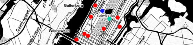
Below are the results of our geocoding and a quick Leaflet map. Enjoy!
# Read in the geocoded data
datgeo <- st_read("data/nyc_superheroes_geo.shp")

# Create the color palette
pal <- colorFactor(
  palette = c("#141dff", "#ff0000", "#00d7ae"),
  domain = datgeo$type
)
# Map the data
leaflet(datgeo) %>%
addProviderTiles(providers$Stamen.Toner) %>%
addCircles(popup = ~name,
radius = ~200,
color = ~pal(type),
fillOpacity = 1,
stroke = FALSE) %>%
addLegend("bottomright", pal = pal, values = ~type,
opacity = 1)
Excellent post. Gained a lot of knowledge from it. Looking ahead for more of such interesting postings